💪 Intro to RL

# Markov Chain (MC)
$$
\mathcal{M}=\{\mathcal{S}, \mathcal{T}\}
$$
$\mathcal{S}$ - state space
- states $s \in \mathcal{S}$ (discrete or continuous)
- 满足Markov Property:
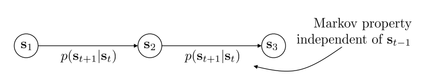
$\mathcal{T}$ - transition operator
- $p\left(s_{t+1} \mid s_t\right)$
## examples
let $\mu_{t, i}=p\left(s_t=i\right)$
$\vec{\mu}_t$ is a vector of probabilities
let $\mathcal{T}_{i, j}=p\left(s_{t+1}=i \mid s_t=j\right)$
then $\vec{\mu}_{t+1}=\mathcal{T} \vec{\mu}_t$
# Markov Decision Process (MDP)
$$
\mathcal{M}=\{\mathcal{S}, \mathcal{A}, \mathcal{T}, r\}
$$
$\mathcal{S}$- state space
- states $s \in \mathcal{S}$ (discrete or continuous)
$\mathcal{A}$ - action space
- actions $a \in \mathcal{A}$ (discrete or continuous)
$\mathcal{T}$ - transition operator (now a **Tensor**)
$r$ - reward function
$$
\begin{aligned}
&r: \mathcal{S} \times \mathcal{A} \rightarrow \mathbb{R} \\
&r\left(s_t, a_t\right)-\text { reward }
\end{aligned}
$$
## example

let $\mu_{t, j}=p\left(s_t=j\right)$
let $\xi_{t, k}=p\left(a_t=k\right)$
let $\mathcal{T}_{i, j, k}=p\left(s_{t+1}=i \mid s_t=j, a_t=k\right)$
$\mu_{t+1, i}=\sum_{j, k} \mathcal{T}_{i, j, k} \mu_{t, j} \xi_{t, k}$
## partially observed MDP

# Goal of RL

$$
\underbrace{p_\theta\left(\mathbf{s}_1, \mathbf{a}_1, \ldots, \mathbf{s}_T, \mathbf{a}_T\right)}_{p_\theta(\tau)}=p\left(\mathbf{s}_1\right) \prod_{t=1}^T \pi_\theta\left(\mathbf{a}_t \mid \mathbf{s}_t\right) p\left(\mathbf{s}_{t+1} \mid \mathbf{s}_t, \mathbf{a}_t\right)
$$
- $\tau$: trajectory: a sequence of states and actions
Goal:
$$
\theta^{\star}=\arg \max _\theta E_{\tau \sim p_\theta(\tau)}\left[\sum_t r\left(\mathbf{s}_t, \mathbf{a}_t\right)\right]
$$
--> ==find a policy $\pi_{\theta}$ that produces trajectories with maximal average (expected) reward==
## finite horizon case: state-action marginal
$$
\begin{aligned}
\theta^{\star} &=\arg \max _\theta E_{\tau \sim p_\theta(\tau)}\left[\sum_t r\left(\mathbf{s}_t, \mathbf{a}_t\right)\right] \\
&=\arg \max _\theta \sum_{t=1}^T E_{\left(\mathbf{s}_t, \mathbf{a}_t\right) \sim p_\theta\left(\mathbf{s}_t, \mathbf{a}_t\right)}\left[r\left(\mathbf{s}_t, \mathbf{a}_t\right)\right]
\end{aligned}
$$
## infinite horizon case: stationary distribution
$$
\theta^{\star}=\arg \max _\theta E_{(\mathbf{s}, \mathbf{a}) \sim p_\theta(\mathbf{s}, \mathbf{a})}[r(\mathbf{s}, \mathbf{a})]
$$

# Algorithms
## anatomy of a RL algorithm

- green module: 计算当前的policy怎么样
- blue module: 更新policy
不同算法的每个Module的侧重点/复杂度不一样
## Value Functions
### Q-function
$$
Q^\pi\left(\mathbf{s}_t, \mathbf{a}_t\right)=\sum_{t^{\prime}=t}^T E_{\pi_\theta}\left[r\left(\mathbf{s}_{t^{\prime}}, \mathbf{a}_{t^{\prime}}\right) \mid \mathbf{s}_t, \mathbf{a}_t\right]
$$
==total reward from taking $\mathbf{a}_t$ in $\mathbf{s}_t$==
### Value functions
$$
\begin{aligned}
&V^\pi\left(\mathbf{s}_t\right)=\sum_{t^{\prime}=t}^T E_{\pi_\theta}\left[r\left(\mathbf{s}_{t^{\prime}}, \mathbf{a}_{t^{\prime}}\right) \mid \mathbf{s}_t\right] \\
&V^\pi\left(\mathbf{s}_t\right)=E_{\mathbf{a}_t \sim \pi\left(\mathbf{a}_t \mid \mathbf{s}_t\right)}\left[Q^\pi\left(\mathbf{s}_t, \mathbf{a}_t\right)\right]
\end{aligned}
$$
==average total reward from $\mathbf{s}_t$==
在$s_{t}$处采取不同$a_{t}$获得的total reward的平均值(期望)
> $E_{\mathbf{s}_1 \sim p\left(\mathbf{s}_1\right)}\left[V^\pi\left(\mathbf{s}_1\right)\right]$ is the $\mathrm{RL}$ objective!
### use Q-functions and value functions
**Idea 1**: 如果我们知道policy $\pi$和Q function $Q^{\pi}(s,a)$, 则我们可以improve $\pi$:
set $\pi(\tilde{a}\mid s) = 1$ if $\tilde{a} = \arg \max _{\mathbf{a}} Q^\pi(\mathbf{s}, \mathbf{a})$
**Idea 2**: compute gradient to increase probability of good actions a:
if $Q^\pi(\mathbf{s}, \mathbf{a})>V^\pi(\mathbf{s})$, then $\mathbf{a}$ is better than average, then modify $\pi(\mathbf{a} \mid \mathbf{s})$ to increase probability of $\mathbf{a}$
> These ideas are very important in RL; we'll revisit them again and again!
## types of algos
Objective目标函数:
$$\theta^{\star}=\arg \max _\theta E_{\tau \sim p_\theta(\tau)}\left[\sum_t r\left(\mathbf{s}_t, \mathbf{a}_t\right)\right]
$$
1. policy gradients: 直接对目标函数求导(w.r.t $\theta$), 并更新$\theta$
2. value-based: 不直接求policy, 而是求<font color='blue'> 最优policy </font>对应的$Q^{\pi}$ and $V^{\pi}$(implicite), 并通过$Q^{\pi}$ and $V^{\pi}$来improve policy
3. actor-critic: 不直接求policy, 而是求<font color='blue'> 当前policy </font>对应的$Q^{\pi}$ and $V^{\pi}$(implicite), 并通过$Q^{\pi}$ and $V^{\pi}$来improve policy
4. Model-based RL: estimate the transition model, and then...
- Use it for planning (no explicit policy)
- Use it to improve a policy
- Something else
## trade-off between RL algos
- Different tradeoffs
- `Sample efficiency` <font color = 'blue'>how many samples do we need to get a good policy</font>
最重要的问题: is the algo on-policy or off-policy?
- off-policy: able to improve the policy without generating new samples from that policy
- on-policy: each time the policy is changed, even a little bit, we need to generate new samples

- `Stability & ease of use`
- does it converge?
- if it converges, to what
- does it converge every time?
<font color = 'red'>why is any of this even a question?? --> RL算法通常不能保证convergence</font>
- Supervised learning: almost always gradient descent
- Reinforcement learning: often not gradient descent

- Different assumptions
- Stochastic or deterministic?
- Continuous or discrete?
- Episodic or infinite horizon?

- Different things are easy or hard in different settings
- Easier to represent the policy?
- Easier to represent the model?
## examples of algos
- Value function fitting methods
- Q-learning, DQN
- Temporal difference learning
- Fitted value iteration
- Policy gradient methods
- REINFORCE
- Natural policy gradient
- Trust region policy optimization
- Actor-critic algorithms
- Asynchronous advantage actor-critic (A3C)
- Soft actor-critic (SAC)
- Model-based RL algorithms
- Dyna
- Guided policy search